Abstract

IT departments typically recognise the damage done by workforce attrition only after it has become irreversible. This paper argues that the cause is structural, not managerial inattention, and examines it for the two technical populations of a Dutch IT department separately: software engineers and system administrators. Webster’s (2008) Dead Sea effect describes how the most capable staff leave first while less mobile staff remain; I extend it with a temporal dimension and show that it runs differently for the two groups. The organisation’s own measurement system hides the effect for years: headcount gradually decreases, systems keep running, and the remaining staff absorb responsibilities that make them look indispensable. By the time quality decline becomes visible in delivery, the department has passed a lock-in point where intervention by hiring backfill comes too late to retain knowledge. I propose a five-phase model of this delayed Dead Sea effect, identify the mechanisms that create the delay, and derive leading indicators that would surface the problem while intervention is still possible. A minimal model of knowledge coverage, with the bus factor of a critical system as its only state variable, makes the lock-in point exact (a system is locked in when nobody is left who can change or recover it) and derives the delay: the gap between losing knowledge and discovering the loss is the inverse of how often that knowledge is needed. It runs differently for the two groups. Engineers lose coverage faster but on the change calendar, where failure is seen within a year or two; administrators lose it more slowly, cannot rebuild it from artefacts, and see it only when an incident strikes, typically years later. A stylised case traces a department through all five phases for both groups. This is theoretical research: the model is analytical, its rates are illustrative, and the case is constructed; no empirical data are used, and the paper closes with a measurement appendix and a research agenda that say what data would test it. It is written for the Dutch market situation, with its collective pay scales, dismissal protection, works-council rights and freelance regulation.

Keywords: workforce attrition; voluntary turnover; Dead Sea effect; knowledge loss; IT management; software engineers; system administrators; Netherlands; bus factor; leading indicators; theoretical model

1. Introduction

The cost of IT attrition is well documented; the timing of its recognition is not. Replacement cost estimates in the practitioner literature run from roughly 90% to 200% of annual salary once recruiting, onboarding and lost productivity are counted. Yet most IT departments monitor attrition through a single lagging number: the annual turnover rate. That number answers how many left, not who left or what left with them.

The gap matters because IT work concentrates tacit knowledge in few heads. A legacy integration, an undocumented deployment ritual, a backup scheme that only one administrator has ever restored from, or a vendor relationship often lives with one or two people. When those people leave, the department does not fail immediately. It degrades slowly, and the degradation is invisible to the metrics that management reads.

Webster (2008) named the selective pattern behind this: in large IT organisations, the strongest technical staff are the most likely to leave, and the least mobile remain. He called it the Dead Sea effect. His essay is widely cited by practitioners but has never been developed into a model, and it says little about when the effect becomes visible.

This paper addresses that gap with one question: why do IT organisations recognise the Dead Sea effect only after the point where it can still be reversed, and what would allow them to recognise it earlier?

Two populations and one market. An IT department has two technical populations that this paper keeps apart from the first page to the last: software engineers, who build and change systems and whose work leaves a trace in version control, and system administrators, who run infrastructure, networks, databases, storage and operations, whose knowledge is procedural and leaves a trace mainly in tickets, on-call rosters and memory. Both groups are subject to the Dead Sea effect. They are not subject to it in the same way: they leave at different rates and by different routes, their knowledge is lost and recovered differently, and the instruments that would detect their loss are different. Collapsing them into one category, as Webster’s essay and most of the practitioner literature do, hides exactly the differences that decide how long the delay lasts. Where this paper gives a figure, a finding or a recommendation, it gives it for each group, and says where they agree.

The paper is written for the Dutch market situation. Four features of it bear directly on the argument and recur throughout. Most large Dutch employers and the whole public sector set technical pay through collective agreements (CAOs) with fixed scales and annual steps, so that salary growth for a strong engineer who stays is slow and predictable, which is the condition under which high performers leave (Section 2.2). Dutch dismissal law requires a preventive review by the UWV or the subdistrict court and a statutory severance, so the staff who remain are hard to move once entrenched. Works councils have a right of consent over systems that monitor staff and over the processing of personnel data, which constrains how the indicators of Section 6 may be built. And the Dutch ICT labour market was classed as very tight in the fourth quarter of 2024 for all three ICT occupation groups the UWV distinguishes (UWV, 2025) and has cooled since, with vacancies falling from their 2023 peak to about 18,900 in the second quarter of 2026 while unemployment among ICT workers has risen (UWV, 2026); the resumption of enforcement against sham self-employment in January 2025 has at the same time narrowed the freelance route that both groups, and administrators especially, used as an exit and that employers used as a substitute for hiring (Minister van SZW & Staatssecretaris van Financiën, 2026). None of these features is unique to the Netherlands, but their combination is, and the paper does not claim that its figures transfer unchanged to other markets.

The argument proceeds as follows. Section 2 reviews the Dead Sea effect, the research literature that supports its core claim, the neighbouring constructs it is often confused with, and the two populations as the Dutch market presents them. Section 3 identifies the mechanisms that delay recognition. Section 4 proposes a five-phase model and Section 5 derives, from a minimal model of knowledge coverage, both the lock-in point and the length of the delay. Section 6 derives leading indicators, Section 7 traces a stylised department through the five phases, Section 8 discusses interventions, and Section 10 sets out limitations and an empirical research agenda. Appendix 12 gives operational definitions for every indicator.

2. Background

2.1 The Dead Sea effect

Webster (2008) observed that the competence distribution of a large IT department should, all else equal, mirror that of its hires, but in practice drifts downward over time. The engineers most able to find work elsewhere leave when they encounter organisational dysfunction; those who remain tend to entrench themselves as maintainers of critical systems, becoming hard to remove. He named the pattern after the Dead Sea, where water leaves only by evaporation and salt is left behind. Webster explicitly framed it as a tendency, not a law: not everyone who stays is “residue”, and well-managed groups avoid the pattern entirely. The essay appeared on his blog as a chapter draft for a book that was never published, and the concept has since spread mainly through practitioner channels.

2.2 Who leaves: the performance–turnover literature

The core claim, that leavers are not a random sample of the workforce, has substantial empirical support. Jackofsky (1984) proposed that voluntary turnover is curvilinear in performance: low performers are pushed out, high performers are pulled out by outside offers, and average performers stay. Trevor, Gerhart and Boudreau (1997) confirmed this in 5,143 employees of a single firm and found that the high-performer end of the curve is driven by salary growth: where salary growth lagged, turnover among top performers was extremely high. Salamin and Hom (2005) replicated the U-shape in Swiss banking. Williams and Livingstone (1994) meta-analysed 55 studies and found that turnover is concentrated among poor performers only where pay is contingent on performance; where it is not, the relationship weakens or disappears.

Two implications follow for IT. First, the Dead Sea effect is the high-performer arm of a well-established curve, not a folk theory. Second, the conditions that produce it are specific: flat salary growth and weak performance differentiation, both common in large corporate and public-sector IT.

2.3 Functional versus dysfunctional turnover

Dalton, Todor and Krackhardt (1982) argued that a raw turnover rate is misleading because it combines functional turnover (poor performers leaving, which helps the organisation) with dysfunctional turnover (good performers leaving who could have been retained). Their taxonomy anticipates the central measurement problem this paper examines: an aggregate turnover figure can look healthy while its composition is destructive.

2.4 What leaves: knowledge loss

DeLong (2004) documented how technology-intensive organisations lose critical tacit knowledge through retirement and unexpected mid-career departures, and showed that the loss typically surfaces months or years after the departure, when a situation arises that only the departed employee knew how to handle. Practitioner work from the same period framed the problem as workforce attrition explicitly; Kaplan (2009) and Manpower (2010) both reported that a substantial share of employers had no process for capturing departing employees’ knowledge.

2.5 Related constructs

The Dead Sea effect sits next to several better-known ideas, and it is worth saying precisely how it differs from each.

Bus factor. The bus factor (or truck factor) of a system is the number of people who would have to leave before the system can no longer be maintained. Software-engineering research has operationalised it from version-control history (Cosentino, Cánovas Izquierdo & Cabot, 2015; Avelino et al., 2016). It is a snapshot of knowledge concentration at a point in time, and its established measures are built on version control, which records what software engineers do but not what administrators do; Appendix 12 extends it to administered systems. The Dead Sea effect is the process that drives the bus factor down; the bus factor is one of its best measurements (Section 6), not a competing explanation.

Brooks’s law. Brooks (1975) observed that adding people to a late software project makes it later, because onboarding and communication overhead outweigh the added capacity. The law concerns a project in time trouble. Section 8 generalises the mechanism to a team in composition trouble: a team that has lost its strongest members lacks the capacity to onboard, so adding people fails for the same reason, permanently rather than for the duration of a project.

Functional and dysfunctional turnover. Dalton et al. (1982) supplied the taxonomy; the Dead Sea effect is the case in which turnover is systematically dysfunctional and the aggregate figure hides it. The contribution here is the temporal argument: why the organisation learns of the dysfunction late.

Organisational forgetting. De Holan and Phillips (2004) distinguish purposeful forgetting from accidental forgetting, and within the latter, the failure to capture new knowledge from the decay of knowledge already held. Knowledge loss through attrition is accidental decay. The Dead Sea effect adds a selection mechanism to this literature: it is not random knowledge that decays but, disproportionately, the knowledge held by those most able to leave.

Absorptive capacity. Cohen and Levinthal (1990) argued that an organisation’s ability to recognise, assimilate and apply new knowledge depends on the related knowledge it already holds. The mechanism in Section 3.5 is absorptive capacity applied to people rather than to information: a team’s capacity to retain a strong hire depends on the strong colleagues already present. In Section 5 this appears as the simple fact that knowledge transfer needs a source: once nobody is left who knows a system, nobody can be taught it.

Turnover theory. A century of turnover research (Hom et al., 2017) has concentrated on individual-level antecedents: why a given person decides to leave. Nyberg (2010) shows that for high performers, pay growth and promotion speed moderate that decision. The present paper takes the individual-level results as given and asks a team-level question: what the sequence of such decisions does to the composition of what remains, and when anyone notices.

2.6 Two populations, two labour markets

The performance–turnover literature treats employees as one population ranked on performance. For the argument here the technical staff of an IT department have to be split in two, because the Dead Sea effect works through three things that differ systematically between software engineers and system administrators: the form their knowledge takes, the route by which they leave, and the trace they leave behind for measurement.

Knowledge. Engineers’ knowledge is partly codified in the artefacts they produce. Code, tests, schemas and pipelines survive their author, badly documented but readable. Administrators’ knowledge is procedural: how to fail over a cluster, which order to restart services in, what the undocumented dependency between the firewall and the batch window is, why the restore has to be done from the second-oldest snapshot. It is acquired by doing and held in memory, and it is exercised on systems whose failure stops the whole business rather than one function. In the terms of Section 5, a strong administrator is harder to replace by a strong hire than a strong engineer is, because there is less to read and more to be shown.

Exit routes in the Dutch market. In the fourth quarter of 2024 the UWV classed all three ICT occupation groups it distinguishes, software and application developers, database and network specialists, and ICT user support, as facing a very tight labour market (UWV, 2025); since then the market has cooled, with ICT vacancies falling steadily from 2023 and the number of ICT workers on unemployment benefit rising to about 6,400 in July 2026, partly through reorganisations in banking (UWV, 2026). Within that common picture the two groups leave by different doors. Strong engineers in a corporate IT department are pulled toward software product companies, scale-ups and consultancies, where pay is set by the market rather than by a CAO scale and where the work is building rather than maintaining. Strong administrators are pulled toward managed-service providers, cloud and hosting companies, and, until recently, toward self-employment: the zzp route was for years the standard way for an experienced Dutch administrator to double their income while doing the same work for the same employer. The lifting of the enforcement moratorium on 1 January 2025 made clients cautious about hiring freelancers for embedded roles (Minister van SZW & Staatssecretaris van Financiën, 2026), which has closed part of that door and, as Section 8 discusses, closed part of the employer’s escape route at the same time.

The side that stays. The Dutch institutional setting also shapes who remains. CAO scales with annual steps mean that a strong engineer or administrator who stays reaches the top of their scale within a few years and then sees no growth, the precise condition under which Trevor et al. (1997) find high-performer turnover to be extremely high. Dismissal protection means that staff who have entrenched themselves cannot readily be moved; the preventive test and the statutory transition payment make the residue of Webster’s metaphor a durable fact rather than a management choice. Both features apply to both groups. The difference is that an entrenched administrator holds the root passwords and the on-call rota, so that entrenchment is operational as well as organisational.

Trace. Finally, the two groups differ in what they leave behind for measurement. Every change an engineer makes is attributed in version control, so knowledge concentration can be computed from history (Appendix 12). An administrator’s work is attributed, if at all, in change tickets, incident records and on-call schedules, which are thinner, less consistently kept and often record who filed rather than who did. The practical consequence runs through the rest of the paper: the effect is harder to see for administrators, and the indicators for them must lean more on asking and less on computing.

Taken together, these literatures establish who leaves, what leaves and which neighbouring ideas are already in use, and this section has set out why the two populations have to be followed separately. None of the literature addresses when the organisation finds out. That is the contribution of the following sections.

3. Why the effect is delayed

The Dead Sea effect is delayed because every signal management receives is either neutral or falsely reassuring until the damage is structural. I identify six mechanisms. They are not independent; together they form a measurement system that is blind to exactly the variable that matters.

3.1 Headcount declines, but slowly. Attrition is only partly backfilled, so headcount drifts down rather than dropping. A department that loses three engineers and hires two reports a net loss of one, a figure small enough to be absorbed into the budget cycle or read as efficiency. The turnover rate, the only attrition metric most IT leaders see, is a count. It cannot distinguish the departure of the person who understood the billing integration from the departure of someone who could be replaced in a week, and a slowly shrinking count hides the fact that what left was disproportionately the top of the distribution. Dalton et al. (1982) made this point in general; in IT, where competence varies by an order of magnitude between individuals, the masking is extreme. For administrators there is a further mask: a larger share of their departures takes the form of planned retirement or internal transfer to a service-management role, which no turnover metric counts as a loss at all.

3.2 Systems keep running. Production software does not stop when its author leaves. The knowledge gap becomes visible only when the system needs to change or fails, which may be months or years later (DeLong, 2004). Until then, the department appears to be delivering as before. For administered systems the point is sharper still: a backup that has never been restored, a certificate renewal done by hand once a year, a firewall rule set nobody else has read, all keep working until the day they do not, and that day may be years after the person who understood them left. Operational stability is read as organisational health when it is in fact momentum. For engineers the latency is set by the change calendar: the gap shows when the system next has to change. For administrators it is set by the failure calendar: the gap shows when the system next breaks, which is rarer and later.

3.3 Residue entrenchment looks like loyalty. Webster noted that those who stay tend to take on the responsibilities nobody else wants and become maintenance experts on critical systems. From management’s chair this reads as commitment and low risk: these are the people who know the systems and never leave. The organisation’s dependency on them grows precisely as its ability to evaluate them shrinks, because the people who could have judged their work have left. For administrators the entrenchment is literal as well as organisational: the remaining administrator holds the privileged accounts, the vendor contacts and the on-call rota, and under Dutch dismissal law is in any case not readily moved. For engineers it takes the form of sole ownership of systems nobody else can build.

3.4 Survivorship in reporting. Information about engineering quality flows upward through engineers. After the strongest engineers leave, the people reporting on the state of the systems, the backlog and the team are the remaining staff, who have no incentive and often no reference point to report decline. Exit interviews, the one channel that captures the leavers’ view, are typically run by HR, aggregated, and read as individual grievances rather than as a pattern. The survivorship is worse for administrators, whose reporting channel is the incident and availability dashboard: an operations team that has lost its best people reports green until the day it reports red.

3.5 Hiring feedback arrives late and is misattributed. When the department finally tries to backfill with strong hires, two things happen. Strong candidates notice the environment during interviews or in the first months and leave again, producing infant attrition. Those who stay are absorbed into the residue’s way of working. Management typically attributes this to a tight labour market or poor recruiting, not to the state of the team the hires are joining. The two groups fail differently here. Strong engineers are found and then lost: they accept, see the environment, and leave within the year. Strong administrators are more often not found at all: the Dutch pool is thinner, the strong ones are already with service providers or were self-employed, and the vacancy stays open for months, which management reads as a market signal rather than a composition signal.

3.6 The feedback loop is self-reinforcing. Each departure of a capable engineer makes the environment less attractive to the next one, raises the load on those remaining, and lowers the quality bar against which new hires are judged. The effect accelerates while every indicator management reads looks tolerable. By the time delivery metrics move, the department has passed what I call the lock-in point: the state in which the remaining team can no longer absorb or retain a strong hire.

The delay, then, is not a failure of attention. It is the predictable output of measuring attrition as a count, reading stability as health, and relying on the survivors for information about what was lost.

Figure 1 draws the six mechanisms as two reinforcing loops and marks where the organisation’s instruments are attached. Both loops run through the departure of strong engineers. The first (R1) runs through workload: each departure raises the load on those remaining and lowers the attractiveness of staying. The second (R2) runs through evaluation: each departure removes someone able to judge work and onboard newcomers, which lowers the quality bar and makes the next strong hire leave early. The instruments management reads, turnover rate, headcount and delivery metrics, are attached to the periphery of the loops, at the points that move last. The variables at the centre, the share of strong engineers and the concentration of knowledge, have no instrument on them at all.

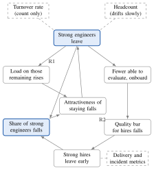
Figure 1. The two reinforcing loops behind the delayed Dead Sea effect and where management’s instruments (dashed) are attached. The variables that decide the outcome (highlighted) have no instrument on them.

4. A stage model of the delayed Dead Sea effect

The mechanisms in Section 3 unfold in a recognisable sequence. I describe it as five phases, distinguished by the gap between what management observes and what is happening in the team (Figure 2). The phases are ordered, not timed: the duration of each depends on the organisation, and I deliberately attach no durations to them.

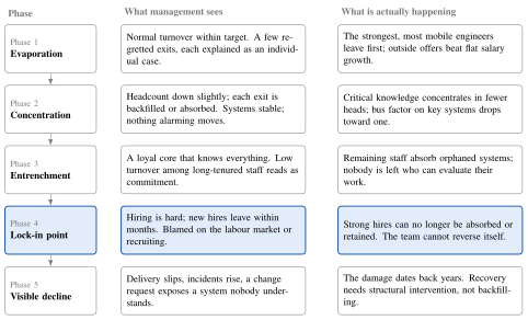
Figure 2. The delayed Dead Sea effect in five phases. Every signal available to management looks tolerable until the lock-in point (Phase 4, highlighted) has passed; the first unambiguous signal arrives in Phase 5.

Phase 4 is the pivot. Before it, the department can still recover through ordinary retention and hiring measures. After it, the remaining team’s norms, load and knowledge gaps prevent strong hires from taking hold, so the same measures fail and are misread as a market problem. Management’s first unambiguous signal (Phase 5) arrives one full phase after the last point at which conventional intervention would have worked.

The two groups pass through the same five phases but show different signatures in each, and the delay between what is happening and what is seen is longer for administrators at every phase (Table 1). The difference is largest in Phases 2 and 5. In Phase 2 an engineering team’s knowledge concentration is at least visible in version control to anyone who looks; an operations team’s is visible only to the team. In Phase 5 an engineering team fails on a change, which is scheduled and therefore seen coming; an operations team fails on an incident, which is not.

Phase	Software engineers	System administrators
1 Evaporation	Senior developers and architects leave for product companies and scale-ups; each exit has a story; pay gap visible in exit interviews.	Senior administrators leave for service providers, cloud companies or (before 2025) self-employment, or retire; retirements are not counted as regretted losses.
Concentration	Bus factor on key codebases drops; visible in commit history to anyone who looks; code keeps running.	Bus factor on infrastructure drops; visible only to the team; procedures handed over in meetings rather than exercised; systems keep running.
Entrenchment	Remaining seniors own the systems nobody else can build; architecture reviews stop; new ideas stall.	Remaining seniors hold privileged access, vendor relationships and the on-call rota; runbooks go stale; nobody outside the team can judge whether operations are sound.
Lock-in	Senior hires are found, join, and leave within the year, citing an inability to change anything.	Senior hires are often not found; vacancies stay open for months; those who join are given systems nobody can explain and leave or conform.
Visible decline	A programme slips or a change request cannot be scheduled; the failure is on the change calendar and is seen approaching.	A restore, failover or upgrade fails; the failure is on the incident calendar and arrives without warning, typically later than the engineering failure.

Table 1. Phase signatures by group: how each phase of Figure 2 presents for software engineers and for system administrators.

The model makes two claims that can be tested. First, the lock-in point exists and is identifiable: for each critical system it is the moment nobody is left who can change or recover it, after which the knowledge can only be rebuilt from artefacts, if there are any. Second, the observable indicators in the left column of Figure 2 stay within tolerable bounds until Phase 5, while measurable team properties in the right column (knowledge concentration, departure quality, early-tenure attrition) move from Phase 1 onward. Section 5 shows that both follow from a model with one state variable.

5. A formal treatment

The stage model is verbal. To check that the delay is a consequence of the mechanisms rather than a rhetorical device, I write down the smallest model that contains them. It has one state variable, the bus factor of a critical system, and four rates. Everything the paper measures (Section 6) and everything the case turns on (Section 7) can be read from it directly, and the difference between the two groups enters as a difference in what knowledge is and how its loss is observed, not as a difference in parameters chosen to fit.

5.1 Setup

Consider one critical system and let $k(t)$ be the number of people who can change or recover it: its bus factor. Four things happen to $k$, each tied to a mechanism of Section 3.

1. Departure. Each knower leaves at hazard $\lambda$ per year, and takes the knowledge with them: $k \to k-1$ at rate $\lambda k$. This is the Dead Sea effect itself; $\lambda$ is the exit hazard of the people who hold critical knowledge, who are, by Webster’s argument and Section 2.2, the strong ones.

2. Transfer. Each knower trains one colleague at rate $\tau$ per year: $k \to k+1$ at rate $\tau k$. Transfer needs a source. When $k = 0$ there is nobody to learn from, which is the lock-in point of Section 4, now exact: a system is locked in when its bus factor reaches zero, because from that state internal transfer is impossible.

3. Rebuilding from artefacts. When $k = 0$, a newcomer can reconstruct the knowledge from what the system left behind, at rate $\alpha$. For software, code, tests and schemas make $\alpha$ appreciable; for administered systems, whose knowledge is procedural, $\alpha$ is close to zero. This is the one structural difference between the groups.

4. Observation. The system is hit, at rate $\mu$ per year, by an event that needs deep knowledge: a change request that touches its internals, or an incident that needs more than a restart. If $k = 0$ when the event arrives, the failure is visible to management; otherwise it is absorbed and nothing is seen. For engineers $\mu$ is the rate of deep changes, for administrators the rate of deep incidents, and the second is lower.

Only the first three rates move $k$; the fourth decides when management finds out. With $\alpha = 0$ the process is a linear birth–death process and the probability that a system with $k_0$ knowers has reached zero by time $t$ has a closed form,

$$P_0(t \mid k_0) = \left[\frac{\lambda\,(1 - e^{-(\lambda-\tau)t})}{\lambda - \tau\, e^{-(\lambda-\tau)t}}\right]^{k_0}, \qquad \lambda > \tau, \tag{1}$$

and, once it is at zero, the expected time until management sees a failure is simply

$$E[\text{recognition delay}] = 1/\mu . \tag{2}$$

Equation (1) says that a system with a sole owner ($k_0 = 1$) is lost with probability $\lambda(1-e^{-(\lambda-\tau)t})/(\lambda - \tau e^{-(\lambda-\tau)t})$, which rises toward one whenever departures outpace transfer; a system with two knowers is lost with the square of that, which is why the Phase 2 indicator in Section 6 is the count of systems at bus factor one. Equation (2) is the delay of the paper’s title in one symbol: the gap between the loss and its recognition is set by how often the lost knowledge is needed, and by nothing else. A department can shorten it only by needing the knowledge on purpose, which is what a disaster-recovery test is.

Rate	Meaning	Eng.	Adm.
$\lambda$	departure of a knower	0.15	0.11
$\tau$	transfer to a colleague, per knower	0.08	0.06
$\alpha$	rebuilding from artefacts when $k=0$	0.20	0.02
$\mu$	deep change or incident on the system	0.40	0.20
	critical systems at start	12	8
	of which at bus factor one	3	1

Table 2. Parameters of the knowledge-coverage model for the two groups. Rates are per year; values are illustrative. The structural difference is in $\alpha$ (codified vs. procedural knowledge) and $\mu$ (change-driven vs. incident-driven observation); the difference in $\lambda$ follows Section 2.6.

5.2 Result: loss first, recognition later, and later still for administrators

Table 1 gives illustrative rates for the two groups and the starting coverage of the case department of Section 7: twelve critical engineering systems, three of them with a sole owner, and eight administered systems, one of them with a sole owner. The values are chosen to be round and to respect three orderings argued in Section 2.6: strong engineers leave faster than strong administrators; code can be read after its author leaves but a procedure cannot; and a change that needs deep knowledge of a given system comes more often than an incident that does. Figure 3 shows what follows, from the closed form for $\alpha = 0$ and from simulation otherwise.

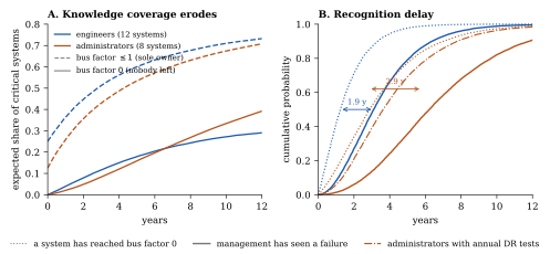
Figure 3. The knowledge-coverage model for the two groups at the parameters of Table 2. (A) Expected share of critical systems with a sole owner (dashed) and with nobody left who can change or recover them (solid). (B) Cumulative probability that at least one critical system has reached bus factor zero (dotted) and that management has seen a failure on one (solid); the arrows mark the median gap between the two, which is the recognition delay. The dash-dot line shows administrators when a disaster-recovery test is run on each critical system once a year.

Panel A is the Phase 2 picture. Coverage erodes from the first year in both groups, and the share of systems with a sole owner, the indicator a composition dashboard would show, passes one half after 2.8 years for engineers and 4.3 years for administrators. The share with nobody left rises more slowly, and here the groups cross: engineers lose systems to zero faster but recover some of them from the code, so their curve flattens at about a quarter of systems; administrators lose more slowly but, with nothing to rebuild from, keep losing, and by year seven have more systems at zero than the engineers.

Panel B is the Phase 5 picture, and the paper’s central claim in a single figure. For engineers the median time to the first zero-coverage system is 1.2 years and the median time to the first visible failure is 3.1 years: a recognition delay of 1.9 years, during which the composition dashboard would have shown the loss and the management dashboard would have shown nothing. For administrators the first zero comes at 2.8 years and the first visible failure at 5.8: a delay of 2.9 years, and a visible failure that arrives almost three years after the engineers’. The administrators’ slower erosion, which makes them look like the stable group, is exactly what makes their failure later, and their lower observation rate is what makes it later still.

Three further results follow from the model and bear on Section 8.

1. Transfer protects the stock, not the sole owners. Doubling the transfer rate $\tau$ keeps the long-run coverage of the department from eroding at all (the one-half trigger is never reached), but barely moves the time to the first zero, because a system with a single owner is in a race between one departure and one handover whatever the department’s average. Knowledge distribution works in Phase 2, on the systems that still have two or more knowers; it cannot rescue the systems already at one.

2. Retention buys time everywhere, but less than one would hope. Cutting the departure hazard by a fifth moves every milestone later by three to twelve months. It does not change the shape of the curves, and in particular does not change the recognition delay, which depends on $\mu$ alone.

3. Observation is a lever, and only administrators need it. Running a disaster-recovery test on each administered system once a year raises their effective $\mu$ from 0.2 to 1.2. It does not slow the loss by a day, but it cuts the median recognition delay from 2.9 years to 0.5, so that the operations team learns of its first lost system in year 3.6 instead of year 5.8, while there is still time to act on the others (dash-dot line in Figure 3B). Engineers do not need this lever, because the change calendar tests their systems for them.

Table 3 collects these results.

Group	Scenario	Trigger (y)	First zero (y)	First visible (y)	Delay (y)	P(visible by year 6)
Engineers	baseline	2.8	1.2	3.1	1.4	0.88
	retention: $\lambda$ 0.15 $\to$ 0.12	4.1	1.6	3.6	1.5	0.79
	transfer: $\tau$ 0.08 $\to$ 0.16	never	1.3	3.2	1.5	0.82
	no artefacts: $\alpha \to 0$	2.8	1.2	2.9	1.3	0.93
Administrators	baseline	4.3	2.8	5.8	2.4	0.48
	retention: $\lambda$ 0.11 $\to$ 0.08	7.4	3.8	6.6	2.4	0.34
	transfer: $\tau$ 0.06 $\to$ 0.12	never	3.0	5.9	2.4	0.42
	annual DR test: $\mu$ 0.2 $\to$ 1.2	4.3	2.8	3.6	0.5	0.79

Table 3. Median outcomes of the knowledge-coverage model under baseline parameters and single-parameter interventions, by group. Trigger: year in which the expected share of critical systems with a sole owner passes one half. First zero: year in which the first critical system reaches bus factor zero. First visible: year in which management first sees a failure. Delay: median gap between the two. Simulation, 20,000 runs.

5.3 What the model does not claim

The model is a sketch, not a calibration. The rates are chosen to be round and correctly ordered, not estimated; systems are treated as independent, although in a real department the same people own several and one departure empties more than one; and “knows the system” is binary where competence is not. What the model does establish does not depend on the values. Given that knowers leave, that transfer needs a source and that the lost knowledge is only needed occasionally, three things follow for any values: the loss precedes its recognition by a gap whose expected length is the inverse of how often the knowledge is needed; systems with a sole owner are the ones that are lost, so the count of them is the leading indicator; and a group whose knowledge is procedural and whose failures are incidents rather than changes will be recognised later than one whose knowledge is in artefacts and whose failures are on the change calendar. The Dutch setting enters through $\lambda$, which the CAO scale raises for the strongest and dismissal law does nothing to lower for the rest, and through the recent closing of the freelance route, which removed the one way an employer had of putting $k$ back to one after it had reached zero.

6. Early-warning indicators

If the model holds, the department should stop watching the turnover rate and start watching the composition and consequences of departures. Each indicator in Table 4 corresponds to a mechanism in Section 3 and moves in the phase shown, well before delivery metrics do.

Indicator	What it measures	Replaces	Phase
Regretted-loss rate	Share of leavers whose manager, asked at exit, would have fought to keep them	Turnover rate	1
Leaver performance quartile	Which performance quartile departures come from, tracked over time	Turnover rate	1
Exit-offer gap	Difference between a leaver’s new salary and current pay, from exit interviews	Nothing (usually not collected)	1
Bus factor per critical system	Number of people who can change or recover each production system without help	Headcount	2
Knowledge-concentration index	Share of critical systems whose bus factor is 1	Headcount	2
Orphaned-system count	Systems whose original author or primary maintainer has left and were reassigned rather than transferred	Nothing	2
Tenure skew	Ratio of staff with over five years’ tenure to staff with under two	Nothing	3
External review frequency	How often code, architecture or operations are evaluated by someone outside the team	Nothing	3
Early-tenure attrition	Share of hires leaving within twelve months, tracked separately from overall attrition	Turnover rate	4
Offer-acceptance rate for senior roles	Share of senior offers accepted, and reasons for declines	Time to hire	4

Table 4. Leading indicators of the delayed Dead Sea effect, the aggregate metric each replaces, and the phase of Figure 2 in which it first moves.

The indicators are the same for both groups; their sources and their reliability are not (Table 2). For engineers the two compositional indicators that matter most in Phase 2, bus factor and knowledge concentration, can be computed from version-control history without asking anyone. For administrators they must be assembled from change and incident records and confirmed by asking, which makes them both more expensive and more easily evaded. Conversely, the Phase 1 indicators are harder for engineers in one respect: a larger share of their departures is to employers who pay by the market, so the exit-offer gap is informative, while for administrators retirements and transfers dilute it and the regretted-loss question has to be asked about departures that the turnover rate does not count at all.

Indicator	Engineers	Administrators
Regretted-loss rate	Exit review by engineering lead	Exit review by operations lead, including retirements and transfers
Leaver quartile	Performance ratings	Performance ratings; often compressed in operations
Exit-offer gap	Exit interview; informative	Exit interview; diluted by retirements, zzp rates not comparable
Bus factor	Version-control history (computed)	Change and incident records plus structured asking
Knowledge concentration	Computed from bus factors	Assembled; confirm by “who could restore this from nothing”
Orphaned systems	Ownership register vs. leaving dates	Same, plus whether procedures were exercised at handover
Tenure skew	HR tenure data	HR tenure data
External review	Architecture and code review log	Audit, DR-test and configuration review log
Early-tenure attrition	Hiring cohorts	Hiring cohorts; small numbers, read with care
Senior offer acceptance	Recruiting records	Recruiting records plus time-to-fill, since vacancies stay open

Table 5. Primary data source for each indicator, by group. The engineers’ sources are mostly computable; the administrators’ mostly require asking.

Operational definitions, data sources and known pitfalls for each indicator are given in Appendix 12. Three observations about the set. First, most indicators are cheap: several require only a different cut of data HR already holds. Second, the indicators in phases 1 and 2 are the ones that matter, since by phase 4 the lock-in point has been reached. Third, the indicators are compositional, not aggregate: they ask who and what, not how many. That is the shift Dalton et al. (1982) called for four decades ago and that IT management reporting has largely not made.

A constructed case

The following case is constructed, not observed. It exists to show what the five phases look like from inside an organisation and to give the model of Section 5 a concrete setting. It is not a report on any employer, and its figures are illustrative rather than measured; its value is that every event in it is one a reader who has worked in corporate IT will recognise.

6.1 Setting

Department R is the internal IT department of a mid-sized Dutch manufacturing company. In year 0 it has 60 technical staff: 36 software engineers in three teams (ERP integration, logistics and warehouse systems, a data platform) and 24 system administrators in two (infrastructure and network; databases, storage and workplace). It maintains about twenty production systems that the business regards as critical, twelve owned by the engineering teams and eight by operations. Turnover has run at 10 to 13% a year for a decade, in line with the company’s other departments. Pay follows the company CAO: fixed scales with annual steps, so that a senior engineer and a senior administrator who stay reach the top of their scale within four or five years and then see no growth. Performance ratings exist but have no effect on pay. Several of the administrators are over fifty.

6.2 The six years

Table 6 summarises what the department’s management dashboard showed in each year and what a composition dashboard, had it existed, would have shown. The phases of Figure 2 are marked.

Year	Headcount, turnover	Management dashboard	Composition dashboard	Phase
0	60, 12%	Baseline. Delivery on plan; incidents within tolerance.	E: regretted-loss rate 15%, BF1 3 of 12. A: regretted-loss rate 10%, BF1 1 of 8. Early-tenure attrition 10% in both.	–
1	58, 13%	Turnover slightly up. Two senior departures, each with a story: the integration architect moved abroad, the platform lead joined a start-up.	E: regretted-loss rate 60%; both leavers top-quartile; exit-offer gap +25%; BF1 6 of 12. A: unchanged.	1 (E)
2	57, 11%	Turnover back to normal. “Most stable year in a while.” Senior storage administrator retires as planned; a senior network administrator goes freelance and is hired back on a day rate. Two engineering backfills made, both junior.	E: regretted-loss rate 50%; BF1 8 of 12; three systems reassigned to the remaining senior engineer without handover. A: regretted-loss rate 0% as recorded (retirement and freelance exit not counted); BF1 4 of 8; backup and restore procedures handed to the network administrator, never exercised.	2 (E), 1 (A)
3	55, 10%	Lowest turnover in five years. Long-tenured core praised for reliability. Delivery on plan; availability 99.9%.	E: no architecture review in the year; tenure skew 3.5 (was 1.2); one senior hire leaves after seven months, early-tenure attrition 50%. A: no DR test in two years; tenure skew 4.0; the freelance network administrator’s contract is ended in January under the DBA enforcement, taking the only current knowledge of the firewall estate with him; BF1 6 of 8.	3 (E), 2 (A)
4	54, 14%	Turnover up because of “market conditions”. Three senior engineers hired; two leave within a year. Senior administrator vacancy open all year. Recruiter engaged.	E: early-tenure attrition 67%; senior offer acceptance 40% (was 75%); BF1 9 of 12. A: time-to-fill for senior roles exceeds twelve months; two offers declined, one accepted and withdrawn; BF1 7 of 8.	4 (E), 3 (A)
5	52, 12%	ERP upgrade slips nine months. A pricing-engine change request cannot be scheduled: nobody can modify the system. Escalation to the board. Availability still 99.8%.	E: the dashboard would show nothing new; the column has been moving for four years. A: BF1 7 of 8; a restore has not been tested in four years; the operations column is still moving and nobody has looked at it.	5 (E), 4 (A)
6	50, 11%	Change work outsourced to a vendor; internal engineering team shrunk. A warehouse database restore fails during a storage migration; the procedure describes an array replaced three years earlier; two days of outage.	A: Phase 5 arrives a year after the engineers’.	5 (A)

Table 6. Department R over six years: what management saw and what a composition dashboard would have shown, by group (E = engineering teams, A = operations teams). Figures are illustrative. BF1 = critical systems with a bus factor of one, out of 12 (E) and 8 (A).

The two groups move through the phases out of step, the engineers roughly one phase ahead throughout, and the department’s management sees one crisis where there are two. The timeline is one plausible path through the model of Section 5 at the parameters of Table 1: Department R’s engineers see their first failure a little later than the model’s median of 3.1 years, its administrators almost exactly at the median of 5.8. In year 1 two of the department’s strongest engineers leave within four months of each other. Each departure has its own explanation and each is accepted on its own terms; nobody asks what they have in common. Both were top-quartile performers, both had been in the same salary band for four years, and both left for a rise of roughly a quarter. The turnover rate rises one percentage point.

Year 2 is quiet. Headcount is down one, turnover is back in range and the systems the two leavers built keep running. The systems they owned are reassigned to the one remaining senior engineer in the integration team, who already owns three others. On the operations side the year looks even quieter. The senior storage administrator retires on schedule, a departure nobody regrets because it was planned; the backup and restore procedures he ran by hand for fifteen years are handed to the network administrator in a two-hour meeting, and are never exercised. The senior network administrator resigns to go freelance and is hired back the following Monday on a day rate for the same work, which the department books as a saving on headcount and the administrator books as a doubling of income; neither appears in the turnover figure as a regretted loss. Two engineering backfills are made at junior grade, because the budget allows two juniors or one senior and two seems safer. The number of critical systems with a single knowledgeable person rises from six to eight on the engineering side and from one to four on the operations side.

Year 3 looks, from the dashboard, like the best year of the period. Turnover is the lowest in five years because the people who would have left have already gone. The long-tenured core is praised in the annual review for stability. One senior engineer is hired into the data platform team and leaves after seven months, citing an inability to get anything changed; the exit interview is filed under “cultural fit”. Nobody outside the department has reviewed its architecture since the integration architect left. In January the company’s legal department, responding to the resumed enforcement of the Wet DBA, ends the freelance network administrator’s contract; he declines an offer to return on a CAO salary at roughly half his day rate, and the firewall estate he alone understood passes to a colleague who has never changed a rule on it. No disaster-recovery test has been run in two years; availability is 99.9% and the operations team is held up as the model of stability.

In year 4 management notices that hiring is hard, and notices it first for the engineers. Three senior engineers are hired; two leave within the year. The explanation offered and accepted is the labour market, and an external recruiter is engaged. Inside the department, the two who left had each been handed a system nobody else understood, with no one able to review their work or answer their questions. The engineering teams have passed the lock-in point: they can no longer retain the people who could reverse their decline. The operations teams show the same phase differently. A senior administrator vacancy is open all year; two candidates decline the offer, one accepts and withdraws before starting after a conversation with the team. Because nobody is hired, nobody leaves early, and the vacancy appears in the recruiting report as a market problem rather than in any attrition figure at all.

In year 5 the engineers’ decline becomes visible. The ERP upgrade, dependent on the integration layer whose architect left four years earlier, slips by nine months. A change request on the pricing engine cannot be scheduled because the single engineer who can modify it is the one carrying six other systems. The matter reaches the board, which is told that the department has an attrition problem. The attrition problem is four years old; what has changed is that it has finally produced a signal management reads. The operations teams, whose availability figure is still 99.8%, are not part of the conversation.

Year 6 brings the default resolution of Section 8 for the engineers: change work moves to a vendor, the internal engineering team shrinks, and the cost of the vendor exceeds what a differentiated retention budget in year 1 would have cost by an order of magnitude. It also brings the operations teams’ Phase 5, a year behind. During a storage migration the warehouse database has to be restored; the restore fails, because the procedure left behind by the storage administrator four years earlier describes an array that was replaced three years earlier, and the only person who had ever run a restore on the new array was the freelance network administrator whose contract was ended in year 3. The warehouse is down for two days. The board, which thought it had dealt with the attrition problem the year before, is told that it has a second one.

6.3 The counterfactual

Suppose Department R had run the composition dashboard of Section 8 from year 0, with the trigger levels proposed there, separately for the two groups. The regretted-loss rate of 60% in year 1 would have breached the one-third trigger in the first quarter after the second departure, forcing a joint review by engineering leadership and HR of what the two leavers had in common. The review would have found the exit-offer gap and the common salary band, and the cheapest intervention available at that point, a retention adjustment for the remaining top-quartile engineers, would have cost roughly a tenth of a senior backfill. Whether it would have been approved is a separate question; the point is that the decision would have been put to someone in year 1 rather than year 5.

Had the first trigger been ignored, the bus-factor count would have breached the one-quarter trigger in year 2, at which point forced knowledge distribution on the eleven single-owner systems was still possible, because the single owners were still there. By year 3 the senior hire who left after seven months would have registered as 50% early-tenure attrition in a cohort of two, a figure small enough to doubt but large enough to prompt the question of why the department could not retain him. On the operations side the triggers would have fired later and more quietly: the regretted-loss question, asked about the retirement and the freelance exit in year 2, would have put the operations teams at 100% regretted loss in a year in which the turnover figure showed nothing; the one-quarter bus-factor trigger would have fired the same year at 4 of 8; and a DR-test trigger, which this paper adds for administered systems in Appendix 12, would have fired in year 3. Each trigger buys the organisation one phase. The case illustrates the model’s central claim: the information needed to act existed at every point, and the organisation’s instruments were simply not pointed at it, and for one of the two groups it was not even collected.

6.4 What the case shows

Four features of the case carry over to real departments. First, every signal in the left-hand column of Table 6 was true and was read correctly as far as it went; the failure was in what was not measured. Second, the year that looked best (year 3) was the last year in which ordinary intervention would have worked for the engineers, and year 4 the last for the administrators. Third, the right-hand column was computable from data the company already held for the engineers, from version control, ratings and hiring records, but for the administrators had to be assembled and asked for, which is why in the case nobody did. Fourth, the two groups ran one phase apart throughout, the administrators’ exits were in forms the turnover rate does not count (retirement, freelancing, an unfilled vacancy), and their Phase 5 arrived after the board believed the problem solved. A department that measures its technical staff as one population will see one crisis and be surprised by the second.

8. Implications for IT management

The practical conclusion is that the timing of intervention matters more than its content. The same measures that reverse the effect in Phase 2 fail in Phase 4.

8.1 Before lock-in

In Phases 1 to 3 the department still contains people capable of evaluating work, absorbing new hires and transferring knowledge. Interventions here are conventional and well supported by the literature:

• Differentiated retention. Trevor et al. (1997) show that salary growth is the strongest lever on high-performer turnover. A retention budget concentrated on the top quartile does more than an across-the-board increase. In a CAO environment the instrument is the labour-market allowance (arbeidsmarkttoelage) or a scale exception, both of which most Dutch collective agreements permit and most IT departments do not use. For engineers the comparison the allowance has to beat is a product-company salary; for administrators, until recently, it was a freelance day rate, which no allowance beats, and since 2025 it is a service-provider salary, which one can.

• Forced knowledge distribution. Pairing, rotation and documentation requirements raise the bus factor on critical systems before anyone leaves. The target is a measurable bus factor of at least two per production system. For engineers this is largely a matter of code review and rotation across codebases. For administrators it is a matter of exercised procedures: a restore, a failover or a certificate rotation that a second person has actually performed under supervision, on a schedule, with the result recorded. A runbook that has not been exercised does not count.

• Exit interviews read as a pattern. Regretted losses should be reviewed together, by engineering leadership rather than HR alone, with the explicit question of what they have in common.

• External evaluation. Periodic review of architecture and code by people outside the team provides the reference point that Section 3.4 shows the team itself loses. For operations the equivalent is a disaster-recovery test observed by someone outside the team, and a configuration review; an availability figure is not a review.

8.2 Sequencing by phase

The formal model of Section 5 gives each intervention a rate to act on, and the stage model gives each a window in which it still works. Table 7 puts the two together. Before the lock-in point, interventions act on the departure hazard $\lambda$, the transfer rate $\tau$ and, for administrators, the observation rate $\mu$; the model shows that transfer protects only systems that still have two or more knowers, that retention buys months rather than years, and that observation is the one lever that shortens the delay itself. After the lock-in point the same levers are still available in principle but there is nothing left to pull them on: knowledge distribution has no source, retention has nobody critical left to retain, and a strong hire assigned to a system at bus factor zero has nobody to learn from and leaves or rebuilds slowly from whatever artefacts exist. The post-lock-in options act instead on the structure of the department, which is why they belong to a different level of management.

Phase	Intervention	Rate	Why it stops working after lock-in
1	Differentiated retention for top-quartile engineers and administrators	$\lambda$	There is no longer a top quartile worth the name; the money goes to the residue and raises its entrenchment.
1	Exit interviews reviewed jointly by engineering and HR as a pattern	$\lambda$ (indirectly)	The leavers are now ordinary performers; the pattern that mattered has already run.
	Forced knowledge distribution: pairing, rotation, exercised handovers per critical system	$\tau$	Transfer needs a source; the systems at bus factor zero have none, and the model shows transfer cannot rescue systems already at one.
2	Senior rather than junior backfill	$\tau$, $\alpha$	A senior hire can only be taught by a remaining knower or rebuild from artefacts; with neither, the hire leaves (Phase 4).
	External review of architecture and code; observed DR tests for administered systems	$\mu$	Still possible, and the one pre-lock-in measure that keeps working; it shortens the delay rather than slowing the loss, and is how the organisation learns it has passed the point.
3	Rebalancing tenure: targeted hiring into the long-tenured core	$\tau$	The core resists; new hires have no source to learn from and leave.
–5	A new nucleus built outside the existing team	structure	–
4–5	Managed decline with frozen scope	structure	–
4–5	External capacity for change work	structure	–

Table 7. Interventions by phase, the model parameter each acts on, and why each stops working after the lock-in point.

8.3 A composition dashboard

The indicators of Section 6 are only useful if someone looks at them together, at the right cadence, with authority to act. Three design choices follow from the model.

Owner. The dashboard belongs to engineering leadership, not HR. HR owns the turnover rate and is the right owner for it, but the composition indicators require engineering judgement (which systems are critical, who is strong) and engineering data (version control). A dashboard that HR compiles and engineering receives repeats the survivorship problem of Section 3.4 in a new form.

Cadence. Quarterly, with a four-quarter rolling window. Annual review is too slow: in the case of Section 7, the lock-in point was reached between two annual reviews. Monthly is too noisy for a department of sixty, where a single departure moves most rates by several points.

Thresholds. Each indicator needs a trigger level agreed in advance, because a level agreed after the fact will be set wherever the current value happens to be. Reasonable starting points, to be adjusted once a department has two years of its own history: a regretted-loss rate above one third; more than a quarter of critical systems at bus factor one; early-tenure attrition above a quarter in any cohort; and any two senior hires in a row leaving within a year. A trigger does not mandate a specific action; it mandates a review by someone outside the department.

8.4 After lock-in

In Phases 4 and 5, backfilling fails for two reasons. The first is Brooks’s (1975) law in a new form: adding people to a team that lacks the capacity to onboard them slows the team down and drives the new people out. The second is that the hire’s quality bar is set by the team they join, so a strong hire either adapts downward or leaves. Three options remain, none cheap:

1. A new nucleus. Build a separate team with its own norms, staffed from outside, and migrate systems to it over time. The existing team is not disbanded but is no longer the organisation’s standard.

2. Managed decline. Accept that the department can maintain but not change, freeze scope accordingly, and plan replacement of systems rather than renewal of the team.

3. External capacity. Move change work to vendors or partners while the internal team retains operations. This is often what happens by default, unrecognised, and it is the most expensive of the three when counted honestly. In the Netherlands this option has narrowed since 2025: the freelance administrator hired back on a day rate, for years the standard way of keeping lost knowledge within reach, is now a sham-self-employment risk for the employer, and the alternative, a managed-service contract, moves the knowledge out of the organisation permanently.

The common thread is that post-lock-in recovery is a structural decision taken at a level above the IT department. The department itself, by definition of lock-in, cannot make it.

9. Discussion: why the delay persists

If the indicators are cheap and the mechanisms are not obscure, why does the delay persist? Part of the answer is that nobody has written the measurement down, which this paper attempts to remedy. But the larger part is that the delay is held in place by features of how organisations are run, and these deserve to be named, because an indicator that cuts against them will be ignored.

Split ownership of the signal. Turnover is an HR metric; delivery is an IT metric. The composition of departures falls between them. HR sees that someone left and why they said they left; engineering sees that a system has become hard to change. Neither sees that these are the same event, because no report joins them. The composition dashboard of Section 8 is, mechanically, a join between two systems of record that are not normally joined.

Cadence mismatch. The effect unfolds over years; management attention is organised in quarters and annual reviews. A slow process observed at a fast cadence looks like noise, and each quarter’s movement is small enough to be attributed to the quarter’s particular circumstances. Dalton et al. (1982) argued four decades ago that turnover should be characterised rather than counted; the argument did not take because characterising requires looking across cadences, and nothing in the annual cycle rewards that.

Each departure gets a story. People leave for reasons, and the reasons are true: a move abroad, a start-up, a partner’s job. The organisation accepts each story because each is accurate. What the stories share, that the leaver was strong, underpaid relative to the market, and able to go, is never the stated reason and is therefore never aggregated. The regretted-loss rate exists to force that aggregation.

Stability is rewarded. Low turnover is read as good management and is often an explicit management target. In the case of Section 7, the year of lowest turnover was the year the department was praised, and it was also the year the lock-in point was crossed. A target on the turnover rate, without a target on its composition, rewards exactly the outcome the model warns against: the strong have left and the rest are staying.

The visible cost arrives in someone else’s budget. The savings from slow backfill and junior hires appear in the department’s own budget in the year they are made. The cost appears years later, in the form of a vendor contract, a slipped programme or a failed change, and is booked to a programme, a vendor line or a one-off. The department that caused the cost is rarely the one charged with it, and the accounting therefore never closes the loop that Figure 1 draws.

The scale is the ceiling. In most large Dutch employers and across the public sector, technical pay is a CAO scale with annual steps. A strong engineer or administrator reaches the top of the scale in a few years, after which the only route to higher pay is promotion out of the technical work or departure. The scale is designed to be fair across the organisation; its effect on the technical population is to guarantee the condition under which the strongest leave. Most CAOs allow exceptions, in the form of a labour-market allowance or placement in a higher scale, and most IT departments do not know this or do not use it.

The residue is protected. Dutch dismissal law requires a reasonable ground, a preventive test by the UWV or the subdistrict court, and a statutory transition payment. This is a feature of the system, not a flaw, but it means that the composition of a team cannot be corrected from the bottom once it has deteriorated; the only remaining lever is the top. Organisations that treat the Dead Sea effect as a performance-management problem, to be solved by removing weak staff, will find in the Netherlands that it cannot be solved that way, and had better prevent it.

The indicators need consent. The indicators of Section 6 process personal data of current and former staff and several of them, the leaver performance quartile and the regretted-loss rating in particular, constitute a system for monitoring performance. Under Article 27 of the Works Councils Act the works council has a right of consent over arrangements for the processing of personnel data and for monitoring staff (Wet op de ondernemingsraden, art. 27 lid 1), and the General Data Protection Regulation requires a documented purpose and a retention schedule. None of this prevents the dashboard; it does mean that building it is a decision taken with the works council, not by engineering leadership alone, and that the data on leavers has a retention period after which it must be aggregated or deleted. A department that wants to start measuring should start that conversation first.

The survivors write the reports. This is Section 3.4 restated as an institutional fact: the people with the least incentive to report decline, and the least ability to see it, are the ones from whom the organisation takes its information about the team. External review (Section 6) is the only remedy, and it is unpopular for the same reason it is necessary.

None of these features is irrational on its own. Together they guarantee that a department will learn about its composition in Phase 5. Changing them is harder than adding indicators, but the indicators are where to start, because they make the features visible.

10. Limitations and further research

This paper is conceptual, and its central construct has an unusual pedigree. The Dead Sea effect was proposed in a practitioner essay, has spread by anecdote and has never been tested. I have grounded its core claim in the performance–turnover literature, but the extension I propose, the delay and the lock-in point, rests on argument, not data. Three limitations follow.

Selection in the evidence. The mechanisms in Section 3 are drawn from cases where the effect occurred and was eventually recognised. Departments that avoided it, or in which capable engineers left without the predicted degradation, do not appear in the practitioner record. The model may therefore overstate how often attrition of strong performers leads to lock-in.

Measurement of “strong”. Both Webster’s essay and this paper assume that engineering competence can be ranked. In practice, performance ratings in IT are noisy, and the people best placed to judge are, by the model’s own logic, the ones who have left. Any empirical test needs a competence measure independent of the team being studied.

Stylisation of the model and the case. The formal model of Section 5 treats systems as independent, knowledge as binary and rates as constant; the case of Section 7 is a composite. Both are devices for showing that the argument is coherent, not evidence that it is true. The three qualitative results of Section 5 do not depend on the rate values; the years quoted do, and in any real department the rates would have to be estimated from the records Appendix 12 describes.

Generalisation. The argument is built on IT departments inside large Dutch organisations, where tacit system knowledge is concentrated, pay follows a collective scale, dismissal is protected and the freelance route has recently narrowed. It may not transfer to software product companies, consultancies or small teams, where the conditions identified in Section 2.2 differ, nor unchanged to markets without collective pay scales or with at-will employment, where the residue of Webster’s metaphor can be removed rather than only prevented. The two-group split is itself a simplification: data engineers, platform engineers and site-reliability engineers sit between the groups, and the paper’s figures for them would have to be worked out separately.

The model yields hypotheses specific enough to be refuted. Table 8 states them with the data each requires.

	Hypothesis	Operationalisation	Data
H1	In IT departments that later show visible decline, the performance quartile of leavers was higher than the department average for at least two years before delivery metrics moved.	Mean quartile of leavers by year vs. department mean; lead time to first delivery-metric breach.	HR ratings, leaving dates, delivery or incident records.
H2	Knowledge concentration (share of critical systems at bus factor one) rises before early-tenure attrition does, which rises before delivery metrics do.	Cross-correlation of the three series at lags of one to four years.	Version-control history, hiring cohorts, delivery records.
H3	The time from a critical system reaching bus factor zero to its first visible failure is longer for administered systems than for software systems, and shortens where DR tests are run.	For each lost system, date of last knower’s departure vs. date of first failure attributed to it; compare groups and test regimes.	Version control, change and incident records, leaving dates, DR-test logs.
H4	Headcount change over the first three years of the process does not discriminate departments that recover from departments that lock in.	Compare headcount trajectories of recovered and locked-in departments over years 1–3.	Headcount by quarter, outcome classification at year 6.
H5	Differentiated retention spending (concentrated on top-quartile performers) reduces top-quartile exit more than the same spend distributed across all staff.	Difference in top-quartile exit hazard between departments using each policy, controlling for market.	Compensation records, ratings, leaving dates.

Table 8. Testable hypotheses derived from the delayed Dead Sea effect, with the operationalisation and data each requires.

Three study designs would test these hypotheses directly:

1. Retrospective composition analysis. For departments that have experienced visible decline, reconstruct the performance quartile and system ownership of every leaver over the preceding years from HR and version-control records. The model predicts that leaver quality fell and knowledge concentration rose several years before delivery metrics moved.

2. Recognition delay by group. For every critical system that reached bus factor zero, measure the time to the first failure attributed to it, and compare software systems with administered systems and tested with untested systems. The model predicts a longer delay for administered systems and a shorter one where disaster-recovery tests are run; a delay that does not shorten with testing would refute the model’s account of observation.

3. Indicator validation. Where the indicators in Section 6 have been collected, test whether they lead delivery and incident metrics, and by how long. This is the study with the most direct management value and the fewest data requirements.

Version-control history is an underused source for all three. Commit authorship, review participation and file ownership over time provide a longitudinal record of who knew what, independent of HR ratings, in exactly the organisations the model describes.

11. Conclusion

IT organisations recognise the Dead Sea effect late because their measurement systems are built to miss it. Turnover is counted rather than characterised, operational stability is read as health, and the people who could report the loss are the ones who have left. I have proposed a five-phase model in which these mechanisms produce a lock-in point one full phase before the first unambiguous signal reaches management, and a set of compositional indicators that would move earlier. The model is testable with data most organisations already hold.

For software engineers the conclusion is that the effect is fast, visible to anyone who looks, and recoverable if caught early. Strong engineers leave quickly for market-paid work, their departure is recorded as attrition, their knowledge is partly in the code, and the composition of the team can be read from version control. In the model the first system is lost at just over a year and the loss is seen at about three, a delay of under two years. The levers are pay and transfer: a differentiated retention budget within the latitude most Dutch collective agreements already allow, and knowledge distribution applied before systems reach a single owner, since the model shows it cannot rescue them afterwards.

For system administrators the conclusion is that the effect is slow, invisible to anyone who does not ask, and harder to recover from. Strong administrators leave more slowly, by routes that the turnover rate does not count (retirement, transfer, until 2025 freelancing, and the unfilled vacancy), their knowledge is procedural and leaves no artefact, and the composition of the team cannot be computed; it has to be assembled from thin records and confirmed by asking. In the model the first system is lost at just under three years and the loss is seen at almost six, a delay of three years that no retention measure shortens, because the delay is set by how rarely the lost knowledge is needed. The lever is practice: exercised handovers, and disaster-recovery tests observed by someone outside the team, which the model shows cut the delay from three years to six months without slowing the loss by a day, and which no engineering team needs because its change calendar does the same job.

For both groups the practical message is the same, and in the Dutch setting it has a particular edge. The question to ask about attrition is not how many left, but who, what they took with them, and whether anyone is left who would notice. In a market where the residue cannot be dismissed and the strongest are paid by a scale, the only time to answer it is before the lock-in point, and the only way to answer it for administrators is to ask.

Appendix A. Measuring the indicators

This appendix gives an operational definition, a data source and the main pitfall for each indicator in Table 4. All can be computed quarterly from records most organisations already keep; none requires a survey.

Regretted-loss rate. At each voluntary departure, the leaver’s manager answers one question, recorded by HR: would you have made a counter-offer to keep this person? The rate is regretted departures divided by all voluntary departures over a rolling four quarters. Pitfall: managers rate retrospectively more generously once a departure is known to have hurt; collect the answer within a week of notice.

Leaver performance quartile. Each leaver’s position in the department’s performance distribution, taken from the mean of their last two ratings before notice. Report the share of leavers from the top quartile. Pitfall: ratings compressed toward the middle hide the signal; where ratings are uninformative, substitute a forced ranking by two managers at exit.

Exit-offer gap. Median percentage difference between the leaver’s new total compensation and their current one, from exit interviews. Pitfall: leavers understate or decline to answer; a response rate below half makes the figure unreliable, and the response rate itself is then the indicator.

Bus factor per critical system. The number of people who could be lost before no one remaining can change or recover the system. For systems under version control it can be computed from history without asking anyone. The method of Avelino et al. (2016) assigns each developer $d$ a degree of authorship for each file $f$,

$$\mathrm{DOA}(d,f) = 3.293 + 1.098\,\mathrm{FA} + 0.164\,\mathrm{DL} - 0.321\ln(1 + \mathrm{AC}),$$

where $\mathrm{FA}$ is 1 if $d$ created the file, $\mathrm{DL}$ is the number of changes $d$ made to it and $\mathrm{AC}$ the number of changes made by others. A developer is counted as knowing a file when their normalised DOA is at least 0.75 of the file’s maximum and the absolute value is at least 3.293. The bus factor is then found by removing developers in order of files known until more than half of the system’s files have no remaining knowledgeable developer. For administered systems, which are mostly outside version control, the same idea is applied to other records of who did what: change-management tickets per system, incident resolutions per system, on-call rotation membership, and, where infrastructure is defined as code, the configuration repository. A person counts as knowing an administered system when they have closed changes or incidents on it in the last year without escalating to someone else. Pitfall: these records are thinner than commit history and often attribute work to whoever filed the ticket rather than whoever did it; for the most critical systems, confirm the computed figure by asking the team to name who could restore the system from nothing, and treat a hesitation as a bus factor of one.

Knowledge-concentration index. The share of critical systems whose bus factor is one. “Critical” should be defined by the business (systems whose outage stops revenue or compliance), not by IT. Pitfall: the index can be gamed by splitting systems; fix the system list for at least a year.

Orphaned-system count. The number of critical systems whose author or primary maintainer has left and which were reassigned to an existing owner without a handover period of at least a month of overlap. For administered systems, count a handover as real only if the new owner has executed the critical procedures (restore, failover, certificate rotation) at least once under supervision; a runbook handed over unexercised is not a handover. Source: system ownership register cross-referenced with leaving dates. Pitfall: ownership registers are rarely maintained; the first computation usually requires reconstructing the register, which is itself informative.

Tenure skew. The ratio of staff with more than five years’ tenure to staff with less than two, computed separately for engineers and administrators. A healthy department renewing itself sits near one; a department whose inflow has dried up or does not stay climbs above two. Pitfall: a reorganisation that moves people between departments resets tenure in some HR systems; use tenure with the employer, not the cost centre.

External review frequency. The number of occasions per year on which code, architecture or operational practice was evaluated by someone outside the team: an architecture review board, a security audit with findings discussed, a peer department’s review, an external consultant’s assessment. Count only reviews that produced written findings. Pitfall: compliance audits that check documents rather than systems should not be counted.

Early-tenure attrition. For each hiring cohort (hires in a given half-year), the share who have left within twelve months of their start date. Report by cohort, not by calendar year, so that the figure for a cohort is known once and does not drift. Pitfall: the figure lags by a year by construction; pair it with the offer-acceptance rate, which does not.

Offer-acceptance rate for senior roles. The share of offers for senior positions that were accepted, over a rolling four quarters, and the recorded reasons for declines. Pitfall: recruiters record the reason that reflects least on the process; ask the candidate directly where possible.

Disaster-recovery test currency (administrators). For each critical administered system, the number of months since a restore, failover or rebuild was last performed end to end by someone other than its primary owner, with the result recorded. This indicator has no engineering counterpart and is added here because the case of Section 7 turns on it. Trigger: any critical system above twelve months, or any system whose last test was performed only by a person who has since left. Pitfall: a test that was started and abandoned is often logged as performed; count only tests with a recorded outcome.

Reading the set. No single indicator is decisive. The pattern the model predicts is a rise in regretted losses and top-quartile exits (phase 1), followed by a fall in bus factor and a rise in orphaned systems (phase 2), followed by a rise in tenure skew and a fall in external review (phase 3), and only then by a rise in early-tenure attrition and a fall in senior offer acceptance (phase 4). A department that sees the first two movements has time; one that sees the last two has very little.

99

Avelino, G., Passos, L., Hora, A., & Valente, M. T. (2016). A novel approach for estimating truck factors. In Proceedings of the 24th IEEE International Conference on Program Comprehension (ICPC), 1–10. https://doi.org/10.1109/ICPC.2016.7503718 (author version: https://homepages.dcc.ufmg.br/~mtov/pub/2016-icpc.pdf)

Becker, W. J., & Cropanzano, R. (2011). Dynamic aspects of voluntary turnover: An integrated approach to curvilinearity in the performance–turnover relationship. Journal of Applied Psychology, 96(2), 233–246. https://doi.org/10.1037/a0021223

Brooks, F. P. (1975). The Mythical Man-Month: Essays on Software Engineering. Addison-Wesley.

Cohen, W. M., & Levinthal, D. A. (1990). Absorptive capacity: A new perspective on learning and innovation. Administrative Science Quarterly, 35(1), 128–152. https://doi.org/10.2307/2393553

Cosentino, V., Cánovas Izquierdo, J. L., & Cabot, J. (2015). Assessing the bus factor of Git repositories. In Proceedings of the 22nd IEEE International Conference on Software Analysis, Evolution, and Reengineering (SANER), 499–503. https://doi.org/10.1109/SANER.2015.7081864

Dalton, D. R., Todor, W. D., & Krackhardt, D. M. (1982). Turnover overstated: The functional taxonomy. Academy of Management Review, 7(1), 117–123. https://doi.org/10.5465/amr.1982.4285499

De Holan, P. M., & Phillips, N. (2004). Remembrance of things past? The dynamics of organizational forgetting. Management Science, 50(11), 1603–1613. https://doi.org/10.1287/mnsc.1040.0273

DeLong, D. W. (2004). Lost Knowledge: Confronting the Threat of an Aging Workforce. Oxford University Press. https://doi.org/10.1093/acprof:oso/9780195170979.001.0001

Hom, P. W., Lee, T. W., Shaw, J. D., & Hausknecht, J. P. (2017). One hundred years of employee turnover theory and research. Journal of Applied Psychology, 102(3), 530–545. https://doi.org/10.1037/apl0000103

Jackofsky, E. F. (1984). Turnover and job performance: An integrated process model. Academy of Management Review, 9(1), 74–83. https://doi.org/10.5465/amr.1984.4277940

Kaplan, B. (2009). Managing the risk of knowledge loss due to workforce attrition. Presentation to the SIKM Leaders Community, June 2009. https://www.slideshare.net/SIKM/managing-the-risk-of-knowledge-loss-due-to-workforce-attrition

Manpower Inc. (2010). Knowledge retention and transfer in the world of work. White paper, announced 13 April 2010. https://investor.manpowergroup.com/node/51361

Minister van Sociale Zaken en Werkgelegenheid & Staatssecretaris van Financiën. (2026, 12 February). Brief aan de Tweede Kamer inzake zelfstandig ondernemerschap: reactie op het position paper van VZN en handhaving op arbeidsrelaties (Kamerstukken II 2025/26, 31 311, nr. 304). https://zoek.officielebekendmakingen.nl/kst-31311-304.pdf

Nyberg, A. (2010). Retaining your high performers: Moderators of the performance–job satisfaction–voluntary turnover relationship. Journal of Applied Psychology, 95(3), 440–453. https://doi.org/10.1037/a0018869

Salamin, A., & Hom, P. W. (2005). In search of the elusive U-shaped performance–turnover relationship: Are high performing Swiss bankers more liable to quit? Journal of Applied Psychology, 90(6), 1204–1216. https://doi.org/10.1037/0021-9010.90.6.1204

Trevor, C. O., Gerhart, B., & Boudreau, J. W. (1997). Voluntary turnover and job performance: Curvilinearity and the moderating influences of salary growth and promotions. Journal of Applied Psychology, 82(1), 44–61. https://doi.org/10.1037/0021-9010.82.1.44. Open-access working paper: https://ecommons.cornell.edu/entities/publication/7dd1115c-022a-4dc6-9af7-7a4a31a0c19a

UWV. (2025, 18 December). Ontwikkeling krapte naar beroep 2024–2030. https://www.uwv.nl/assets-kai/files/3dadda9c-258e-4d9f-b60c-eac75496816b/ontwikkeling-krapte-naar-beroep-2024-2030.pdf

UWV. (2026, 8 October). ICT-beroepen: arbeidsmarktinformatie. https://www.uwv.nl/nl/arbeidsmarktinformatie/sector/ict

Webster, B. F. (2008, 11 April). The wetware crisis: The Dead Sea effect. Bruce F. Webster (blog). https://brucefwebster.com/2008/04/11/the-wetware-crisis-the-dead-sea-effect/

Wet op de ondernemingsraden, art. 27. https://wetten.overheid.nl/BWBR0002747

Williams, C. R., & Livingstone, L. P. (1994). Another look at the relationship between performance and voluntary turnover. Academy of Management Journal, 37(2), 269–298. https://doi.org/10.2307/256830